From Pixels to Probabilities

How a CNN Sees and Understands an Image

↓

1

Input Image (Pixels)

The journey begins with raw pixel data — a 3D tensor of numbers representing height, width, and color channels (RGB).

What the network receives

A grid of numbers between 0-255 (or 0-1 normalized)
Three channels: Red, Green, Blue
Spatial structure: pixels next to each other are related
Typical size: 224x224x3 for classification

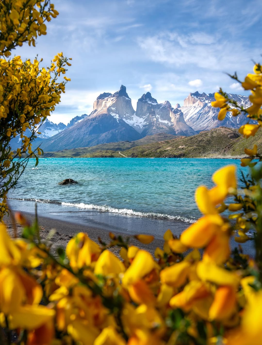
Torres del Paine, Patagonia — 224x224x3 tensor

"The network sees numbers, not pictures — every pixel is just a number with no inherent meaning."

⚡

Interactive: How Convolution Works

A kernel slides over the input image in 3D, computing weighted sums at each position. The result is a feature map that highlights specific patterns.

⟶

Output Feature Map

Each cell shows the result of the kernel applied at that position — highlighting where the pattern was found

Select a kernel and press Animate to begin

Input Image

Kernel (filter)

Output Feature Map

2

Convolution Layer 1 (Edges)

The first layer learns to detect simple, low-level features: edges, corners, and basic gradients.

What is learned at this stage

Horizontal and vertical edges
Diagonal lines and corners
Simple color contrasts
Basic gradient directions

"Each filter responds to one specific pattern — the network learns which patterns are useful."

3

Convolution Layer 2 (Textures)

The second layer combines edges to recognize textures and repeating motifs — surfaces, fabrics, natural patterns.

What is learned at this stage

Rock surfaces, grass, water textures
Repeating patterns and motifs
Surface roughness and smoothness
Regular vs. irregular structures

"Deeper layers learn complex patterns by combining simpler ones — edges become textures."

4

Convolution Layer 3 (Shapes & Parts)

This layer recognizes shapes and identifiable parts of objects — peaks, tree outlines, architectural forms.

What is learned at this stage

Geometric shapes (circles, triangles, rectangles)
Object parts (wheels, eyes, mountain peaks)
Spatial combinations of textures
Boundary contours of objects

"Parts of objects — not whole objects yet. The network now sees structure, not just pattern."

5

Convolution Layer 4 (Objects)

The deepest convolutional layer recognizes entire objects and large-scale structures in the image.

What is learned at this stage

Full objects (mountains, trees, buildings, animals)
Scene composition and layout
Object relationships and context
High-level semantic understanding

"The network now understands 'what' is in the image — full semantic comprehension."

6

Global Pooling (High-Level Features)

Global average pooling collapses each feature map into a single value — summarizing spatial information into a compact vector.

What happens at this stage

Each feature map (e.g., 7x7) becomes a single number
512 feature maps become a 512-dimensional vector
Spatial location is discarded
Only "what" remains, not "where"

→

"Everything the network knows about the image, compressed into one compact vector."

7

Fully Connected + Softmax (Probabilities)

The feature vector is passed through fully connected layers, then softmax converts raw scores into a probability distribution over all classes.

What happens at this stage

Feature vector becomes class scores (logits)
Softmax: e^score / sum of all e^scores
All probabilities sum to 1.0
Highest probability = model's prediction

Mountain landscape82%

Alpine lake8%

Forest landscape5%

Coastal landscape3%

Urban landscape2%

"Probabilities sum to 1.0 — the highest probability is the model's prediction: Mountain landscape (82%)."

Key Takeaways

The hierarchical nature of feature learning in CNNs

▧

Simple to Complex

Early layers learn simple, universal patterns (edges, textures) that appear in any image domain.

◈

Local to Global

Deeper layers learn task-specific, complex concepts — from shapes to full objects and scenes.

▦

Spatial to Semantic

Global pooling discards location; fully-connected layers map features to meaning (class probabilities).

Transfer Learning

Reusing pretrained knowledge for new tasks

VGG16 — Pretrained on ImageNet

1000 classes · 1.2M images

Conv Block 1 — Edges

Conv Block 2 — Textures

Conv Block 3 — Shapes

Conv Block 4 — Parts

Conv Block 5 — Objects

FC Layers (4096)

Softmax (1000 classes)

⟶ Surgery

Fine-tuned for Melanoma Detection

2 classes · 10K images

Conv Block 1 — Edges

Conv Block 2 — Textures

Conv Block 3 — Shapes

Conv Block 4 — Skin Patterns

Conv Block 5 — Lesion Features

New FC Layer (256)

Softmax (Benign / Malignant)

Why It Works

Early layers learn universal features (edges, textures, shapes) that are useful across ALL image domains. No need to relearn them.

What to Freeze

Freeze conv blocks 1-3 (universal features). Fine-tune blocks 4-5 to adapt to domain-specific patterns. Replace the classification head entirely.

Benefits

Less training data needed. Faster convergence. Better generalization. Avoids overfitting on small datasets — critical for medical imaging.